 Mathew K Analytics
Lesson 9 · Mastering Pandas
Hands-On With Pandas: Creating and Exploring DataFrames
In this lesson, we dive into pandas basics and intermediate techniques. Explore how to create, manipulate, and analyze tables of data using Python. Pandas…
- CourseMastering Pandas
- Lesson9 of 44
- Video22 min
- FormatJupyter notebook · 24 code cells
What you'll learn
Data
No separate download needed — the notebook creates or downloads everything it uses.
📓 Full notebook
Download .ipynbHands-On With Pandas: Creating and Exploring DataFrames#
In this lesson, we dive into pandas basics and intermediate techniques. Explore how to create, manipulate, and analyze tables of data using Python.
What is pandas?#
Pandas is a Python library for working with tabular data. It helps you load, clean, explore, and analyze large datasets efficiently.
import warnings
warnings.filterwarnings("ignore")

# First, import pandas with the standard nickname.
import pandas as pd
import numpy as np
np.random.seed(42)
Creating Your First DataFrame#
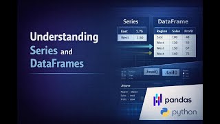
A DataFrame is like a table in Excel: rows and columns with labels. Let's build a simple DataFrame from scratch.
data = {
    "Name": ["Alice", "Bob", "Charlie"],
    "Age": [25, 32, 28],
    "City": ["London", "Paris", "Berlin"]
}
df_small = pd.DataFrame(data)
print(df_small)
Loading Real-World Data: The Titanic Dataset#
We often need to load data from an online data file. The Titanic dataset is a classic example for data analysis.
import pandas as pd
url = 'https://raw.githubusercontent.com/datasciencedojo/datasets/master/titanic.csv'
df = pd.read_csv(url)
print(df.shape)
print(df.head(3))
# Let us see what columns exist and the types of data inside.
print(df.columns)
print(df.dtypes)
# Peek at the last five rows to see other samples.
print(df.tail())
Data Cleaning: Handling Missing Data#
Real-world data is often messy. We must identify and handle missing values before analysis.
# Check for missing values in each column.
print(df.isnull().sum())
# Drop rows where the "Age" column is missing.
df_clean = df.dropna(subset=["Age"])
print(f"Rows before: {df.shape[0]}, after: {df_clean.shape[0]}")
# Fill missing "Embarked" values with the most common port.
most_common_port = df["Embarked"].mode()[0]
df_filled = df.fillna({"Embarked": most_common_port})
print(df_filled["Embarked"].isnull().sum())
Selecting Data: Rows and Columns#
You often want just a part of the table. pandas makes it easy to access columns or rows with simple labels or positions.
# Get all the names of passengers.
names = df["Name"]
print(names.head(5))
# Select rows where passengers are female and under 18.
young_females = df[(df["Sex"] == "female") & (df["Age"] < 18)]
print(young_females[["Name", "Age", "Sex"]].head())
Sorting and Descriptive Statistics#
Sorting data and getting summary stats help us spot patterns quickly.
# Sort by Age from youngest to oldest.
sorted_by_age = df.sort_values("Age")
print(sorted_by_age[["Name", "Age"]].head(5))
# Show summary statistics for numeric columns.
print(df.describe())
# How many unique ticket classes and what are they?
print(df["Pclass"].unique())
print(df["Pclass"].value_counts())
Grouping and Aggregating Data#
Grouping helps you see big patterns, like survival rates for different groups.
# What percent of men and women survived?
grouped = df.groupby("Sex")["Survived"].mean()
print((grouped * 100).round(2))
# What is the average age for each ticket class?
avg_age_per_class = df.groupby("Pclass")["Age"].mean()
print(avg_age_per_class.round(1))
Combining Columns: Creating New Features#
Sometimes, you need to make new columns by combining or transforming others.
# Create a "FamilySize" column (siblings/spouses + parents/children + self).
df["FamilySize"] = df["SibSp"] + df["Parch"] + 1
print(df[["Name", "FamilySize"]].head(5))
Merging DataFrames: Join Two Tables#
Use merging for cases like joining passengers with extra info from another file or dataset.
# Make a toy table with titles by name.
titles = pd.DataFrame({
    "Name": ["Alice", "Bob", "Charlie"],
    "Title": ["Ms", "Mr", "Dr"]
})
merged = pd.merge(df_small, titles, on="Name", how="left")
print(merged)
Pivot Tables: Quick Summaries by Group#
Pivot tables quickly summarize data with one line per group.
pivot = pd.pivot_table(df, index="Pclass", columns="Sex", values="Survived", aggfunc="mean")
print(pivot.round(2))
Time Series: Handling Dates and Plotting Trends#
The Titanic dataset does not have real dates, so let us try the Flights dataset for this.
import seaborn as sns
df_flight = sns.load_dataset('flights')
print(df_flight.shape)
print(df_flight.head(3))
# Convert year and month to a datetime and plot passenger trends.
df_flight["Date"] = pd.to_datetime(df_flight["year"].astype(str) + "-" + df_flight["month"].astype(str) + "-01")
df_flight = df_flight.sort_values("Date")
df_flight.set_index("Date")["passengers"].plot(title="Monthly Flight Passengers")

Pandas Visualization: Quick Charts#
You can plot right from pandas to quickly explore patterns.
df["Age"].plot(kind="hist", bins=30, title="Age Distribution")

Mini-Project: Titanic Passenger Analysis#
Let us use all the skills so far on the Titanic data for a quick analysis.
# Input: Which ticket class do you want to explore?
class_choice = input("Enter a ticket class (1, 2, 3): ")
subset = df[df['Pclass'] == int(class_choice)]
print(f"Number of passengers in class {class_choice}: {subset.shape[0]}")
# What percent of passengers survived in your chosen class?
survival_rate = subset['Survived'].mean() * 100
print(f"Survival rate: {survival_rate:.1f}%")
# List top 3 youngest survivors in your ticket class.
youngest = subset[subset['Survived'] == 1].sort_values('Age').head(3)
print(youngest[['Name', 'Age']])
Best Practices and Performance Tips#
- Use .copy() to avoid changing the original data by accident.
- Avoid loops: most manipulations are faster with built-in pandas methods.
- For very big data, use .read_csv() with options like chunksize and dtype.
- Profile your code with %timeit or %%time to check for slow spots.
Troubleshooting: Common pandas Errors#
- KeyError: Misspelled or missing column. Check spelling and existance.
- SettingWithCopyWarning: You probably edited a slice of the DataFrame. Try using .copy().
- DtypeWarning: Data format is not consistent. Specify data types with dtype when loading.
Challenge: Can You...#
- Find the oldest passenger in each ticket class?
- Plot a bar chart of survived vs. not survived for each class?
- Merge a new table of your own with extra info per person? Pause the video and try one or more!
Recap: What Did You Learn?#
- Creating and loading DataFrames
- Cleaning, selecting, grouping, joining and visualizing data
- Running analyses on real datasets
- Building confidence for your own Python data projects!
Thanks for learning pandas! If you enjoyed this lesson, please like and subscribe for more practical data science videos. Happy coding!
Found this useful?
All lessons, notebooks and datasets here are free. If they helped you, a coffee keeps new lessons coming.
Related lessons
 18 min
Track Fitness & Health Data with Python Pandas | Hands-On Project
 18 min
Analyse E-Commerce Orders with Python Pandas | Full Project Tutorial
 17 min
Build a Personal Finance Budget Tracker in Python with Pandas
 24 min