 Mathew K Analytics
Lesson 17 · Probability and Statistics in python
Understanding Bootstrapping for Estimation and Confidence Intervals in Statistics
Welcome! In this lesson, we will explore how bootstrapping helps us estimate statistics and confidence intervals from data. We will use small, relatable…
- CourseProbability and Statistics in python
- Lesson17 of 35
- Video16 min
- FormatJupyter notebook · 17 code cells
What you'll learn
Data
No separate download needed — the notebook creates or downloads everything it uses.
📓 Full notebook
Download .ipynbBootstrapping for Estimation and Confidence Intervals#
Welcome! In this lesson, we will explore how bootstrapping helps us estimate statistics and confidence intervals from data.
We will use small, relatable examples and a popular real dataset.
By the end, you will know how to apply bootstrapping to your own projects!
import warnings; warnings.filterwarnings("ignore")
# We suppress warnings to keep things clear for beginners.

import numpy as np
import pandas as pd
import seaborn as sns
import matplotlib.pyplot as plt

sns.set_theme()
What is Bootstrapping?#
Bootstrapping is a way to estimate statistics, such as the mean or median, by taking repeated samples with replacement from your data.
We repeat this many times, which helps us understand the variability in our estimates.
It is especially useful when we do not know the true distribution of the data.
Let us start with a simple example.
# Simulating a small example: scores on a quiz out of 10
quiz_scores = np.array([6, 7, 8, 8, 9, 10, 7, 6])
print("Original quiz scores:", quiz_scores)
# Let's compute the sample mean (average) using numpy
sample_mean = np.mean(quiz_scores)
print("Sample mean:", sample_mean)
Why Do We Need Bootstrapping?#
The sample mean can change a lot if we have more or fewer students.
Bootstrapping shows us how much our estimate might vary if we sampled again and again.
# Bootstrapping: resample our data with replacement
np.random.seed(42)
boot_means = []
for _ in range(1000):
    boot_sample = np.random.choice(quiz_scores, size=len(quiz_scores), replace=True)
    boot_means.append(np.mean(boot_sample))
# Convert list to numpy array for easier math
boot_means = np.array(boot_means)
# Plotting the distribution of bootstrapped means
plt.figure(figsize=(8, 4))
plt.hist(boot_means, bins=20, color='orange', edgecolor='k', alpha=0.7)
plt.axvline(sample_mean, color='blue', linestyle='dashed', label='Sample mean')
plt.xlabel("Mean score")
plt.ylabel("Count")
plt.title("Distribution of Bootstrapped Means")
plt.legend()
plt.show()

Calculating a 95% Confidence Interval#
A confidence interval shows the range where we expect the true mean to be, most of the time.
With bootstrapping, we take the 2.5th and 97.5th percentiles of our bootstrapped means.
# Calculate 95% confidence interval from bootstrap samples
lower, upper = np.percentile(boot_means, [2.5, 97.5])
print("95% confidence interval for the mean:", (lower, upper))
Bootstrapping with a Real Dataset#
Now, let us use a popular real dataset to practice bootstrapping. We will use the tips dataset, which contains information about meals, tips, and servers.
Bootstrapping works especially well when we cannot assume the data is normal.
# Data setup
tips = sns.load_dataset("tips")
print("Shape:", tips.shape)
print(tips.head())
# Let's look at total_bill and plot the distribution
plt.figure(figsize=(7, 4))
plt.hist(tips['total_bill'], bins=25, color='skyblue', edgecolor='gray')
plt.xlabel("Total bill ($)")
plt.ylabel("Number of meals")
plt.title("Distribution of Total Bill Amounts")
plt.show()

# Bootstrapping the mean total_bill
np.random.seed(42)
bootstrap_means = []
for _ in range(2000):
    sample = np.random.choice(tips['total_bill'], size=len(tips), replace=True)
    bootstrap_means.append(np.mean(sample))
bootstrap_means = np.array(bootstrap_means)
# Plotting bootstrap means for total_bill
plt.figure(figsize=(8, 4))
plt.hist(bootstrap_means, bins=30, color='green', edgecolor='black', alpha=0.7)
plt.axvline(np.mean(tips['total_bill']), color='red', linestyle='--', label='Dataset mean')
plt.xlabel("Mean of total_bill ($)")
plt.ylabel("Count")
plt.title("Bootstrapped Means for Total Bill")
plt.legend()
plt.show()

# Calculating a 95% bootstrap confidence interval for total_bill mean
ci_low, ci_high = np.percentile(bootstrap_means, [2.5, 97.5])
print(f"We are 95% confident the true mean total_bill is between ${ci_low:.2f} and ${ci_high:.2f}")
# Bootstrapping a median and its confidence interval
medians = []
for _ in range(2000):
    sample = np.random.choice(tips['total_bill'], size=len(tips), replace=True)
    medians.append(np.median(sample))
medians = np.array(medians)
lower_median, upper_median = np.percentile(medians, [2.5, 97.5])
print(f"95% CI for the median total_bill: ${lower_median:.2f} to ${upper_median:.2f}")
Bootstrapping for Difference in Means#
Suppose we want to know if smokers pay more for a meal than non-smokers.
Bootstrapping can estimate the difference in mean total_bill between two groups.
# Split the dataset by smoker status
smokers = tips[tips['smoker']=='Yes']['total_bill'].values
nonsmokers = tips[tips['smoker']=='No']['total_bill'].values

np.random.seed(42)
diffs = []
for _ in range(2000):
    boot_s = np.random.choice(smokers, size=len(smokers), replace=True)
    boot_ns = np.random.choice(nonsmokers, size=len(nonsmokers), replace=True)
    diff = np.mean(boot_s) - np.mean(boot_ns)
    diffs.append(diff)
diffs = np.array(diffs)

ci_diff_low, ci_diff_high = np.percentile(diffs, [2.5, 97.5])
print(f"95% CI for the difference in means: ${ci_diff_low:.2f} to ${ci_diff_high:.2f}")
# Interactive: Estimate your own confidence interval!
value_str = input("Enter a value (mean or median) you want to estimate a CI for [mean/median]: ")
n_trials = int(input("How many bootstrap trials? (e.g., 1000): "))

results = []
np.random.seed(1)
for _ in range(n_trials):
    s = np.random.choice(tips['total_bill'], size=len(tips), replace=True)
    if value_str == 'mean':
        results.append(np.mean(s))
    elif value_str == 'median':
        results.append(np.median(s))
    else:
        continue
results = np.array(results)
interval = np.percentile(results, [2.5, 97.5])
print(f"95% CI for {value_str}: {interval[0]:.2f} to {interval[1]:.2f}")
# Mini-project: Bootstrap the tip proportion for big bills
# Let's see the percentage of bills over $30 that give a tip above 20%
big = tips[tips['total_bill'] > 30]
prop_high_tip = []
np.random.seed(7)
for _ in range(1000):
    sample = big.sample(frac=1, replace=True)
    percent_high = np.mean(sample['tip'] / sample['total_bill'] > 0.2)
    prop_high_tip.append(percent_high)
prop_high_tip = np.array(prop_high_tip)
ci_low, ci_high = np.percentile(prop_high_tip, [2.5, 97.5])
print(f"95% CI for the proportion: {ci_low:.3f} to {ci_high:.3f}")
Best Practices and Troubleshooting#
- Check if your sample is big enough to represent the population.
- Make sure you use enough bootstrap replications (at least 1000 is common).
- Plot your results to check for surprising patterns.
- Always set a random seed for reproducible science.
- When bootstrapping groups, keep group sizes the same as the samples.
Practice with different datasets to become comfortable!
# Extra tip: Bootstrap confidence intervals for the correlation
x = tips['total_bill']
y = tips['tip']
corrs = []
np.random.seed(21)
for _ in range(999):
    idx = np.random.choice(len(x), size=len(x), replace=True)
    corrs.append(np.corrcoef(x.iloc[idx], y.iloc[idx])[0,1])
corrs = np.array(corrs)
ci_corr_low, ci_corr_high = np.percentile(corrs, [2.5, 97.5])
print(f"95% CI for correlation: {ci_corr_low:.2f} to {ci_corr_high:.2f}")
# Challenge: Use bootstrapping to estimate the 95th percentile of total_bill
# (And its confidence interval)
np.random.seed(55)
percentile_95 = []
for _ in range(1000):
    bsamp = np.random.choice(tips['total_bill'], size=len(tips), replace=True)
    percentile_95.append(np.percentile(bsamp, 95))
percentile_95 = np.array(percentile_95)
ci_p95_low, ci_p95_high = np.percentile(percentile_95, [2.5, 97.5])
print(f"95% CI for 95th percentile: {ci_p95_low:.2f} to {ci_p95_high:.2f}")
Recap: Bootstrapping Boosts Our Confidence#
- Bootstrapping lets us estimate uncertainty for any statistic, not just the mean.
- It does not require the data to be normal.
- Confidence intervals tell us how much our estimates can vary.
Keep practicing, try new datasets, and use these skills in your own projects!
Thank you for learning bootstrapping and confidence intervals with us!
If you enjoyed this lesson, give the video a thumbs up and subscribe for more hands-on stats tutorials.
Practice what you learned and let us know which topic you want next. Happy bootstrapping!
Found this useful?
All lessons, notebooks and datasets here are free. If they helped you, a coffee keeps new lessons coming.
Related lessons
 16 min
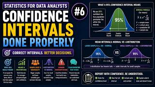
Confidence Intervals Done Properly | Statistics #6
 16 min
Understanding Summarization and Descriptive Statistics in Data Mining
 23 min
Seasonal Patterns in Financial Markets: Understanding Recurring Trends
 17 min