 Mathew K Analytics
Lesson 34 · Probability and Statistics in python
Understanding Bayesian Statistics: Foundations of Priors and Posteriors Explained
Welcome to your first hands-on lesson in Bayesian statistics! We will explore what priors and posteriors mean, why Bayes' rule matters, and how to use…
- CourseProbability and Statistics in python
- Lesson34 of 35
- Video24 min
- FormatJupyter notebook · 13 code cells
What you'll learn
Data
No separate download needed — the notebook creates or downloads everything it uses.
📓 Full notebook
Download .ipynbIntroduction to Bayesian Statistics: Priors and Posteriors#
Welcome to your first hands-on lesson in Bayesian statistics!
We will explore what priors and posteriors mean, why Bayes' rule matters, and how to use Python to run simple Bayesian updates.
By the end, you will build intuition for Bayesian thinking that is useful for science, medicine and AI.
Let us get started!
# Suppress warnings and import basic libraries
import warnings; warnings.filterwarnings("ignore")
import numpy as np
import pandas as pd
import matplotlib.pyplot as plt
import seaborn as sns
np.random.seed(42)

# Set a style for our plots
sns.set(style="whitegrid")
# Data setup: Toy coin-flip dataset
np.random.seed(42)
coin_flips = np.random.binomial(n=1, p=0.5, size=30)
df = pd.DataFrame({'flip': coin_flips})
print("Coin flip outcomes:")
print(df.head())
print(f'Total flips: {len(df)}\nHeads: {df.flip.sum()}  Tails: {len(df) - df.flip.sum()}')
What is a probability?#
Probability is how likely something is.
For a coin flip, we say the chance is 0.5 or 50% for heads, and the same for tails.
Probability in Python is often between 0 and 1.
Let us start exploring these concepts using simple tools.
# Calculate the proportion of heads and tails
prob_heads = df.flip.mean()
prob_tails = 1 - prob_heads
print(f"Proportion heads: {prob_heads:.2f}")
print(f"Proportion tails: {prob_tails:.2f}")
Introducing priors: What if you have some idea before seeing data?#
A prior is your belief about the chance before looking at new evidence.
With a coin, maybe you believe it is a fair coin, or maybe you doubt that.
In Bayesian statistics, we write down our prior as a distribution.
Let us see it in action!
# Define a prior: Beta distribution for a coin's fairness
from scipy.stats import beta
x = np.linspace(0, 1, 101)
prior_a, prior_b = 1, 1  # Uniform prior (no preference)
prior_pdf = beta.pdf(x, a=prior_a, b=prior_b)
plt.figure(figsize=(6,2))
plt.plot(x, prior_pdf, label='Prior: Beta(1,1)')
plt.xlabel('Probability of heads')
plt.ylabel('Plausibility')
plt.title('Uniform Prior Belief: Any Coin Fairness Is Possible')
plt.legend()
plt.show()

What are likelihood and posterior?#
In Bayesian statistics:
- Likelihood = how likely the data is, given each possible probability.
- Posterior = our new belief after seeing the data.
The posterior combines the prior and the data using Bayes' rule.
Next, we will update our belief about this coinstep by step.
# Update: observe our data and calculate the posterior
n_heads = df.flip.sum()
n_tails = len(df) - n_heads
posterior_a = prior_a + n_heads
posterior_b = prior_b + n_tails
posterior_pdf = beta.pdf(x, a=posterior_a, b=posterior_b)
plt.figure(figsize=(6,2))
plt.plot(x, prior_pdf, label='Prior: Beta(1,1)', linestyle=':')
plt.plot(x, posterior_pdf, label=f'Posterior: Beta({posterior_a},{posterior_b})')
plt.xlabel('Probability of heads')
plt.ylabel('Plausibility')
plt.legend()
plt.title('Bayesian Update: Posterior after Seen Data')
plt.show()

# Show the most likely value after updating: mode of the posterior
from scipy.stats import mode
mode_prob = (posterior_a - 1) / (posterior_a + posterior_b - 2) if posterior_a + posterior_b > 2 else 0.5
print(f"Estimated coin fairness (posterior mode): {mode_prob:.2f}")
Priors are flexible: Try other examples#
Some people may start with strong beliefs. For example:
- If you trust the coin heavily, use Beta(10,10)
- If you are very sure it is biased to heads, use Beta(20,5)
Your choice of prior affects what happens, especially with little data.
Let us see a new prior and how the update changes shape!
# Try a different prior: Beta(10,10)
prior2_a, prior2_b = 10, 10
prior2_pdf = beta.pdf(x, a=prior2_a, b=prior2_b)
posterior2_a = prior2_a + n_heads
posterior2_b = prior2_b + n_tails
posterior2_pdf = beta.pdf(x, a=posterior2_a, b=posterior2_b)
plt.figure(figsize=(6,2))
plt.plot(x, prior2_pdf, label='Prior: Beta(10,10)', linestyle=':')
plt.plot(x, posterior2_pdf, label=f'Posterior: Beta({posterior2_a},{posterior2_b})')
plt.xlabel('Probability of heads')
plt.ylabel('Plausibility')
plt.legend()
plt.title('New Prior: Stronger Fair Coin Belief')
plt.show()

Real-life Example: Bayesian model in medicine#
Suppose doctors want to estimate the chance a patient has a disease.
They may start with a prior based on experience.
Each new test result acts as data to update their belief.
This is why Bayesian methods are so useful: they combine what you know and what you see.
# Practice: try your own coin flips and priors
user_heads = int(input("How many heads did you observe? "))
user_tails = int(input("How many tails? "))
user_a = int(input("Set prior 'a' (e.g. 1): "))
user_b = int(input("Set prior 'b' (e.g. 1): "))
user_posterior_a = user_a + user_heads
user_posterior_b = user_b + user_tails
user_posterior_mode = (user_posterior_a - 1) / (user_posterior_a + user_posterior_b - 2) if user_posterior_a + user_posterior_b > 2 else 0.5
print(f"Posterior mode (most likely fairness): {user_posterior_mode:.3f}")
Bayesian inference and uncertainty#
Unlike a single number, Bayesian inference gives us a full range of possible answers.
We see how likely each possible fairness is after our update.
Let us look at the spread, not just the most likely value.
# Plot posterior and show 90% credible interval
lower = beta.ppf(0.05, a=posterior_a, b=posterior_b)
upper = beta.ppf(0.95, a=posterior_a, b=posterior_b)
plt.figure(figsize=(6,2))
plt.plot(x, posterior_pdf, label='Posterior')
plt.axvline(lower, color='red', linestyle='--', label='5% Lower')
plt.axvline(upper, color='blue', linestyle='--', label='95% Upper')
plt.xlabel('Probability of heads')
plt.title('Posterior with 90% Credible Interval')
plt.legend()
plt.tight_layout()
plt.show()
print(f"90% Bayesian credible interval: [{lower:.2f}, {upper:.2f}]")

# Simulate: shrink interval with more flips
df2 = pd.DataFrame({ 'flip': np.random.binomial(1, 0.6, 100) })
n_heads2 = df2.flip.sum()
n_tails2 = len(df2) - n_heads2
posterior_a2 = 1 + n_heads2
posterior_b2 = 1 + n_tails2
lower2 = beta.ppf(0.05, a=posterior_a2, b=posterior_b2)
upper2 = beta.ppf(0.95, a=posterior_a2, b=posterior_b2)
plt.figure(figsize=(6,2))
plt.plot(x, beta.pdf(x, a=posterior_a2, b=posterior_b2), color='green', label='Posterior (100 flips)')
plt.axvline(lower2, color='red', linestyle='--', label='5% Lower')
plt.axvline(upper2, color='blue', linestyle='--', label='95% Upper')
plt.xlabel('Probability of heads')
plt.title('Credible Interval Shrinks with More Data')
plt.legend()
plt.tight_layout()
plt.show()
print(f"90% credible interval with 100 flips: [{lower2:.2f}, {upper2:.2f}]")

Recap: Priors, posteriors, and Bayesian thinking#
Bayesian statistics lets us start with our own beliefs and update them as we see data.
The key terms:
- Prior: what you believe before data
- Likelihood: how likely you would see this data
- Posterior: your new belief after combining both
Now you can apply Bayesian reasoning to coins, medicine, and science problems!
# Practice Challenge: Change priors, sample sizes, or true probability and observe effects
true_p = float(input("Set coin's true probability of heads (e.g. 0.7): "))
n = int(input("How many flips? "))
prior_a = int(input("Set your prior a: "))
prior_b = int(input("Set your prior b: "))
df3 = pd.DataFrame({ 'flip': np.random.binomial(1, true_p, n) })
n_heads3 = df3.flip.sum()
n_tails3 = n - n_heads3
posterior_a3 = prior_a + n_heads3
posterior_b3 = prior_b + n_tails3
xgrid = np.linspace(0,1,101)
plt.figure(figsize=(6,2))
plt.plot(xgrid, beta.pdf(xgrid, a=posterior_a3, b=posterior_b3), label='Posterior')
plt.xlabel('Probability of heads')
plt.title(f'Posterior after {n} flips (true p={true_p:.2f})')
plt.legend()
plt.show()

# YouTube call to action: Like and subscribe!
print("If you enjoyed this intro, please like and subscribe for more data science lessons!")
Found this useful?
All lessons, notebooks and datasets here are free. If they helped you, a coffee keeps new lessons coming.
Related lessons
 15 min
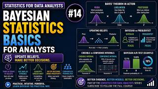
Bayesian Statistics Basics for Analysts | Statistics #14
 16 min
Discrete Distributions Explained: Binomial & Poisson | Statistics #2
 13 min
Simple Linear Regression Explained | Statistics #11
 14 min