 Mathew K Analytics
Lesson 38 · Mastering Pandas
Mastering Time-Based Grouping and Aggregations in Pandas for Effective Data Analysis
In this lesson, we will unlock the power of Pandas for handling time-series data. You will learn how to group, resample, and aggregate data by dates,…
- CourseMastering Pandas
- Lesson38 of 44
- Video20 min
- FormatJupyter notebook · 16 code cells
What you'll learn
Data
No separate download needed — the notebook creates or downloads everything it uses.
📓 Full notebook
Download .ipynbTime-Based Grouping and Aggregations with Pandas#
In this lesson, we will unlock the power of Pandas for handling time-series data.
You will learn how to group, resample, and aggregate data by dates, months, or years.
We will use the classic 'Flights' dataset. This dataset contains airline passenger numbers over time.
By the end, you will build your own mini time-series analysis in Python!
import warnings; warnings.filterwarnings("ignore")
# Data setup (Airline Passenger Flights Dataset)
import seaborn as sns
import numpy as np
np.random.seed(42)
df = sns.load_dataset('flights')
print(df.shape)
print(df.head(3))
Why Time-Based Grouping?#
Many real-life datasets track things over time: sales, weather, traffic, or stock prices.
We want to answer questions like:
- How many passengers flew each year?
- Which month is the busiest?
- Are there seasonal trends?
To do this, we need to group and summarize by time with Pandas.
# Check the columns and data types
print(df.dtypes)

# Preview the columns
print(df.columns)
# Combine 'year' and 'month' into a single datetime column
import pandas as pd
df['date'] = pd.to_datetime(df['year'].astype(str) + '-' + df['month'].astype(str) + '-01')
print(df[['year', 'month', 'date']].head())
# Sort data by date just in case
df = df.sort_values('date')
print(df.head(3))
Visualizing Time-Series Data: First Look#
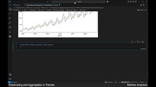
Before grouping or aggregating, it is helpful to draw a simple time-series chart.
This quickly shows any patterns, outliers, or trends in the data.
import matplotlib.pyplot as plt
# Plot the number of passengers over time
plt.figure(figsize=(10,4))
plt.plot(df['date'], df['passengers'], marker='o', linestyle='-')
plt.title('Monthly Air Passengers Over Time')
plt.xlabel('Date')
plt.ylabel('Number of Passengers')
plt.tight_layout()
plt.show()

# Group by year to see total flights per year
yearly = df.groupby('year')['passengers'].sum().reset_index()
print(yearly)
# Find the month with the highest average passengers
monthly_avg = df.groupby('month')['passengers'].mean().sort_values(ascending=False)
print(monthly_avg)
Using Datetime as Index#
Setting datetime as the index unlocks powerful time-based features: resampling, shifting, rolling, and more.
Let us make 'date' the index for our DataFrame.
# Set date as the index
df_ts = df.set_index('date')
print(df_ts.head(3))
# Resample by year and sum passengers
annual = df_ts['passengers'].resample('Y').sum()
print(annual)
# Calculate moving average over 12 months
df_ts['rolling_mean'] = df_ts['passengers'].rolling(window=12).mean()
print(df_ts[['passengers', 'rolling_mean']].head(15))
# Plot original vs. rolling mean
plt.figure(figsize=(10,4))
plt.plot(df_ts.index, df_ts['passengers'], label='Original', color='blue')
plt.plot(df_ts.index, df_ts['rolling_mean'], label='12-Month Moving Avg', color='red')
plt.title('Passengers: Original vs. 12-Month Moving Average')
plt.xlabel('Date')
plt.ylabel('Passengers')
plt.legend()
plt.tight_layout()
plt.show()

Mini-Project: Find Peak Travel Season#
Let us combine what you have learned.
Your task:
Find the month and year when air travel peaked.
Tip: You can use idxmax() and loc to solve this in code!
# Solution: Find the date with max passengers
peak_month = df_ts['passengers'].idxmax()
peak_value = df_ts['passengers'].max()
print(f'Peak month: {peak_month.strftime("%Y-%m")}, Passengers: {peak_value}')
# Group passengers by quarter
quarterly = df_ts['passengers'].resample('Q').mean()
print(quarterly.head())
# Add a column for year and month name (with dt accessor)
df_ts['year'] = df_ts.index.year
df_ts['month_name'] = df_ts.index.month_name()
print(df_ts[['year', 'month_name', 'passengers']].head())
# Aggregate: Find average passengers per year per month
pivot = df_ts.pivot_table(index='year', columns='month_name', values='passengers', aggfunc='mean')
print(pivot.head())
Troubleshooting Tips#
- If your resample gives errors, double-check that your index is datetime.
- If you get missing data or NaN, inspect your data for gaps.
- Always preview your new tables after any operation.
Learning to fix common bugs makes you a real pandas pro!
# Speed tip: Use categorical dtype for month_name if you will use it often
df_ts['month_name'] = pd.Categorical(df_ts['month_name'], categories=['January','February','March','April','May','June','July','August','September','October','November','December'], ordered=True)
print(df_ts['month_name'].head())
Recap: What Did You Learn?#
- How to create datetime columns and sort by date
- Grouping and aggregating by year, month, or quarter
- Resampling, moving averages, and pivot tables for time-series
- Troubleshooting index and data-type issues
With these tools, you can explore trends in almost any time-based data!
Next Steps: Like, Comment, and Subscribe!#
Practice these ideas with your favorite datasetssales, weather, or personal logs.
Let us know in the comments what time-series you want to tackle next.
For more data skills, make sure to like and subscribe for future lessons!
Found this useful?
All lessons, notebooks and datasets here are free. If they helped you, a coffee keeps new lessons coming.
Related lessons
 14 min
Master Data Cleaning and Preparation with Pandas in Python for Effective Bible Study Analysis
 31 min
Comparing SQL and Pandas for Effective Financial Reporting and Data Analysis
 12 min
Mastering Resampling and Aggregation of Time Series Data with Pandas in Python
 12 min