import pandas as pd
import numpy as np
import matplotlib.pyplot as plt
import seaborn as sns
import warnings
warnings.filterwarnings('ignore')
np.random.seed(42) # Set seed for reproducibility

# Beginner Example 1: Create a synthetic banking transactions DataFrame
n_transactions = 1000
n_customers = 200
df = pd.DataFrame({
    'transaction_id': range(1, n_transactions + 1),
    'customer_id': np.random.choice([f'CUST_{i:04d}' for i in range(1, n_customers + 1)], n_transactions),
    'amount': np.round(np.random.normal(150, 60, n_transactions), 2),
    'transaction_type': np.random.choice(['Debit', 'Credit'], n_transactions),
    'channel': np.random.choice(['ATM', 'Online', 'Branch', 'POS'], n_transactions),
    'date': pd.date_range(start='2024-01-01', periods=n_transactions, freq='h')
})
print(df.head(3))

# Beginner Example 2: Check time ordering and data types
print(df.dtypes)
print('Are transactions sorted by date? ', df['date'].is_monotonic_increasing)

# Beginner Example 3: Plot transactions over time
df['date'] = pd.to_datetime(df['date'])
df.set_index('date', inplace=True)
daily_counts = df['transaction_id'].resample('D').count()
plt.figure(figsize=(10,4))
sns.lineplot(data=daily_counts, marker='o')
plt.title('Number of Transactions per Day')
plt.xlabel('Date')
plt.ylabel('Transaction Count')
plt.grid(True)
plt.show()

# Intermediate Example 1: Aggregate transaction amounts by day
daily_amounts = df['amount'].resample('D').sum()
print(daily_amounts.head())

# Intermediate Example 2: Plot aggregated daily transaction amounts
plt.figure(figsize=(10,4))
sns.lineplot(data=daily_amounts)
plt.title('Total Transaction Amount per Day')
plt.xlabel('Date')
plt.ylabel('Total Amount')
plt.grid(True)
plt.show()

# Intermediate Example 3: Calculate rolling 7-day average of daily amounts
rolling_avg = daily_amounts.rolling(window=7).mean()
plt.figure(figsize=(10,4))
sns.lineplot(data=daily_amounts, label='Daily')
sns.lineplot(data=rolling_avg, label='7-Day Average')
plt.title('Transaction Amount with Rolling 7-Day Average')
plt.xlabel('Date')
plt.ylabel('Amount')
plt.legend()
plt.grid(True)
plt.show()

# Intermediate Example 4: Plot monthly seasonality in transaction count
monthly_counts = df['transaction_id'].resample('M').count()
plt.figure(figsize=(8,4))
sns.barplot(x=monthly_counts.index.strftime('%Y-%m'), y=monthly_counts.values)
plt.title('Transaction Counts by Month')
plt.xlabel('Month')
plt.ylabel('Transaction Count')
plt.xticks(rotation=45)
plt.show()

# Advanced Example 1: Detect days with unusually high or low transaction volumes
mean_amt = daily_amounts.mean()
std_amt = daily_amounts.std()
anomaly_days = daily_amounts[(daily_amounts > mean_amt + 2 * std_amt) | (daily_amounts < mean_amt - 2 * std_amt)]
print('Anomolous transaction days:')
print(anomaly_days)

# Advanced Example 2: Add a weekday column, analyze transaction patterns by day of week
df['weekday'] = df.index.day_name()
weekday_amounts = df.groupby('weekday')['amount'].mean().reindex([
    'Monday', 'Tuesday', 'Wednesday', 'Thursday', 'Friday', 'Saturday', 'Sunday'])
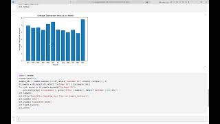
sns.barplot(x=weekday_amounts.index, y=weekday_amounts.values)
plt.title('Average Transaction Amount by Weekday')
plt.xlabel('Weekday')
plt.ylabel('Avg Amount')
plt.show()

# Advanced Example 3: Fill missing dates and check for missing days (data quality)
all_days = pd.date_range(df.index.min(), df.index.max(), freq='D')
filled = daily_amounts.reindex(all_days)
missing_days = filled[filled.isna()]
print('Missing days:', missing_days.index.strftime('%Y-%m-%d').tolist())

# Error Handling Example: What if date column is not datetime?
df_reset = df.reset_index()
df_reset['date'] = df_reset['date'].astype(str)
try:
    df_reset['date'] = pd.to_datetime(df_reset['date'])
    print('Conversion successful!')
except Exception as e:
    print('Error in conversion:', e)

# Error Handling Example: Handling missing values with interpolation
filled_interpolated = filled.interpolate()
plt.figure(figsize=(10,4))
sns.lineplot(data=filled_interpolated, label='Interpolated Totals')
plt.title('Daily Transaction Totals (Interpolated)')
plt.grid(True)
plt.legend()
plt.show()

# Best Practice Example: Always keep raw data untouched, work with copies!
df_raw = df.copy(deep=True)
print('Are df and df_raw equal? ', df.equals(df_raw))

# Best Practice: Use resample or groupby, not for-loops, for time-based analysis
debit_daily = df[df['transaction_type'] == 'Debit']['amount'].resample('D').sum()
credit_daily = df[df['transaction_type'] == 'Credit']['amount'].resample('D').sum()
plt.figure(figsize=(10,4))
sns.lineplot(data=debit_daily, label='Debit')
sns.lineplot(data=credit_daily, label='Credit')
plt.title('Daily Debit vs Credit Totals')
plt.xlabel('Date')
plt.ylabel('Total Amount')
plt.legend()
plt.grid(True)
plt.show()

# End-to-End Example: Detect unusual cash outflow for one customer
target_customer = df['customer_id'].value_counts().idxmax()
cust_df = df[df['customer_id'] == target_customer]
debit_cust = cust_df[cust_df['transaction_type'] == 'Debit']
cust_daily = debit_cust['amount'].resample('D').sum()
window = 7
rolling_mean = cust_daily.rolling(window).mean()
anomaly = cust_daily[cust_daily > rolling_mean + 2 * cust_daily.std()]
print(f'Customer {target_customer} outflow anomalies:')
print(anomaly if not anomaly.empty else 'No anomalies detected.')

# End-to-End Example: Save a plot of this customer's cash outflow
plt.figure(figsize=(10,4))
sns.lineplot(data=cust_daily, label='Daily Outflow')
sns.lineplot(data=rolling_mean, label='7-Day Rolling Mean', linestyle='--')
plt.scatter(anomaly.index, anomaly.values, color='red', label='Anomaly Day', zorder=5)
plt.title(f'Daily Cash Outflow for {target_customer}')
plt.xlabel('Date')
plt.ylabel('Debit Total')
plt.legend()
plt.grid(True)
plt.tight_layout()
plt.savefig('customer_outflow.png')
print('Plot saved as customer_outflow.png')