import pandas as pd
import numpy as np
import matplotlib.pyplot as plt
import seaborn as sns
import warnings
warnings.filterwarnings('ignore')
np.random.seed(42)

# --- Synthetic Transaction Data Setup ---
n_transactions = 1000
n_customers = 200

df = pd.DataFrame({
    'transaction_id': range(1, n_transactions + 1),
    'customer_id': np.random.choice([f'CUST_{i:04d}' for i in range(1, n_customers + 1)], n_transactions),
    'amount': np.round(np.random.normal(150, 60, n_transactions), 2),
    'transaction_type': np.random.choice(['Debit', 'Credit'], n_transactions),
    'channel': np.random.choice(['ATM', 'Online', 'Branch', 'POS'], n_transactions),
    'date': pd.date_range(start='2024-01-01', periods=n_transactions, freq='h')
})

print(df.shape)
print(df.head(3))

print('Nulls in each column:')
print(df.isnull().sum())
print('Duplicates:', df.duplicated().sum())
print('Data types:')
print(df.dtypes)

# --- Convert date to datetime (if needed) and make it the index ---
df['date'] = pd.to_datetime(df['date'])
df = df.set_index('date')
print(df.index.name)
print(df.iloc[:2, :])

# --- Beginner Example 1: Daily Sum of Transactions ---
daily_sum = df['amount'].resample('D').sum()
plt.figure(figsize=(10, 4))
plt.plot(daily_sum)
plt.title('Total Transaction Amount per Day')
plt.ylabel('Amount ($)')
plt.xlabel('Date')
plt.show()

# --- Beginner Example 2: Average Daily Transaction Value ---
daily_avg = df['amount'].resample('D').mean()
print(daily_avg.head(7))

# --- Beginner Example 3: Count of Transactions Per Day ---
daily_count = df['amount'].resample('D').count()
plt.figure(figsize=(10, 3))
plt.bar(daily_count.index, daily_count.values)
plt.title('Number of Transactions Per Day')
plt.ylabel('Count')
plt.xlabel('Date')
plt.tight_layout()
plt.show()

# --- Intermediate Example 1: Weekly Trend Visualization ---
weekly_sum = df['amount'].resample('W').sum()
plt.figure(figsize=(10, 4))
plt.plot(weekly_sum, marker='o')
plt.title('Total Transaction Amount per Week')
plt.ylabel('Amount ($)')
plt.xlabel('Week Starting')
plt.grid(True)
plt.show()

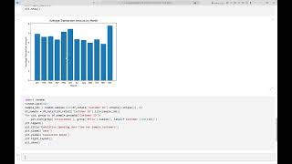
# --- Intermediate Example 2: Detecting Seasonality by Day of Week ---
df['weekday'] = df.index.day_name()
weekday_avg = df.groupby('weekday')['amount'].mean().reindex(['Monday','Tuesday','Wednesday','Thursday','Friday','Saturday','Sunday'])
plt.figure(figsize=(8, 4))
sns.barplot(x=weekday_avg.index, y=weekday_avg.values)
plt.title('Average Transaction Amount by Weekday')
plt.ylabel('Average Amount ($)')
plt.xlabel('Day of Week')
plt.show()

# --- Intermediate Example 3: Rolling 7-Day Total Moving Average ---
rolling_total = daily_sum.rolling(window=7).mean()
plt.figure(figsize=(10, 4))
plt.plot(daily_sum, label='Daily Total')
plt.plot(rolling_total, color='red', label='7-Day Moving Average')
plt.title('7-Day Moving Average of Daily Transaction Amount')
plt.ylabel('Amount ($)')
plt.xlabel('Date')
plt.legend()
plt.show()

# --- Advanced Example 1: Outlier Detection in Transaction Amounts ---
q1 = daily_sum.quantile(0.25)
q3 = daily_sum.quantile(0.75)
iqr = q3 - q1
outlier_upper = q3 + 1.5 * iqr
outlier_lower = q1 - 1.5 * iqr
outlier_days = daily_sum[(daily_sum > outlier_upper) | (daily_sum < outlier_lower)]
print('Outlier Days:')
print(outlier_days)

# --- Advanced Example 2: Heatmap of Transactions by Day and Hour ---
df['hour'] = df.index.hour
pivot = pd.pivot_table(df, values='amount', index='weekday', columns='hour', aggfunc='mean').reindex(['Monday','Tuesday','Wednesday','Thursday','Friday','Saturday','Sunday'])
plt.figure(figsize=(14,4))
sns.heatmap(pivot, cmap='YlGnBu')
plt.title('Average Transaction Amount: Day of Week vs Hour of Day')
plt.ylabel('Day of Week')
plt.xlabel('Hour of Day')
plt.show()

# --- Advanced Example 3: Decompose Trend and Seasonality Components ---
from statsmodels.tsa.seasonal import seasonal_decompose
decompose_result = seasonal_decompose(daily_sum, model='additive', period=7)
decompose_result.plot()
plt.suptitle('Trend, Seasonal, Residual: Daily Transaction Totals')
plt.show()

# --- Error Handling: Missing Dates Example ---
broken_df = df.copy()
broken_df = broken_df.drop(broken_df.index[0])  # simulate a missing date
try:
    broken_df['amount'].resample('D').sum()
except Exception as e:
    print('Error:', e)

# --- Debugging: Detecting Duplicate Transactions ---
duplicate_count = df.duplicated().sum()
print(f'Duplicate transaction rows: {duplicate_count}')

# --- Debugging: Ensuring Datetime Index is Sorted ---
if not df.index.is_monotonic_increasing:
    print('Index out of order; sorting...')
    df = df.sort_index()
else:
    print('Index already sorted!')

# --- End-to-End Banking Problem: Identify Peak Transaction Day and Segment Behavior ---
peak_day = daily_sum.idxmax()
peak_value = daily_sum.max()
print(f'Highest transaction volume day: {peak_day.date()} (${peak_value:.2f})')

# Analyze which transaction type was most common on peak day:
df_peak = df[df.index.date == peak_day.date()]
type_counts = df_peak['transaction_type'].value_counts()
print('Transaction Types on Peak Day:')
print(type_counts)

# Plot hour-by-hour transaction counts for the peak day:
hourly_counts = df_peak.groupby(df_peak.index.hour)['amount'].count()
plt.figure(figsize=(8,3))
plt.bar(hourly_counts.index, hourly_counts.values)
plt.title('Hourly Transaction Counts (Peak Day)')
plt.xlabel('Hour')
plt.ylabel('Count')
plt.tight_layout()
plt.show()