 Mathew K Analytics
Lesson 6 · Python for Data Analysts
End-to-End Data Analyst Capstone
One messy, realistic dataset, taken all the way from raw and broken to cleaned, analyzed, visualized, and reported. This capstone assumes you've already…
- CoursePython for Data Analysts
- Lesson6 of 12
- Video32 min
- FormatJupyter notebook · 29 code cells
What you'll learn
Data
No separate download needed — the notebook creates or downloads everything it uses.
📓 Full notebook
Download .ipynbEnd-to-End Data Analyst Capstone#
- One messy, realistic dataset, taken all the way from raw and broken to cleaned, analyzed, visualized, and reported.
- This capstone assumes you've already covered pandas, numpy, and matplotlib or seaborn basics; we're combining all of it into one real project.
Before You Start#
- Open a new Jupyter Notebook in VS Code and select your Python interpreter as the kernel.
- If anything's missing, open a terminal in VS Code and run: pip install pandas numpy matplotlib seaborn openpyxl
Part 1: The Business Question#
Scenario#
- We're handed a raw export of a small retailer's transactions, and asked one question: which regions and categories are actually driving revenue?
- The export is realistically messy: missing prices, missing regions, duplicate rows, and a handful of obvious data-entry error outliers.
- We'll generate that messy export ourselves, with a fixed seed, so it's reproducible, then clean and analyze it exactly as if it had landed in our inbox.
import numpy as np
import pandas as pd
import matplotlib
matplotlib.use('Agg')
import matplotlib.pyplot as plt
import seaborn as sns

sns.set_theme(style='whitegrid')
print('Libraries ready')
rng = np.random.default_rng(seed=13)
n = 500

regions = ['North', 'South', 'East', 'West']
categories = ['Electronics', 'Home Goods', 'Apparel', 'Sporting Goods']

dates = pd.date_range('2023-01-01', '2023-12-31', periods=n)
customer_ids = rng.integers(1000, 1200, size=n)
region_col = rng.choice(regions, size=n)
category_col = rng.choice(categories, size=n)
quantity_col = rng.integers(1, 6, size=n)
unit_price_col = rng.uniform(8, 200, size=n).round(2)

raw = pd.DataFrame({
    'transaction_id': range(1, n + 1),
    'date': dates,
    'customer_id': customer_ids,
    'region': region_col,
    'category': category_col,
    'quantity': quantity_col,
    'unit_price': unit_price_col,
})
print(raw.shape)
messy = raw.copy()

missing_price_idx = rng.choice(n, size=20, replace=False)
messy.loc[missing_price_idx, 'unit_price'] = np.nan

missing_region_idx = rng.choice(n, size=15, replace=False)
messy.loc[missing_region_idx, 'region'] = None

outlier_idx = rng.choice(n, size=8, replace=False)
messy.loc[outlier_idx, 'unit_price'] = messy.loc[outlier_idx, 'unit_price'] * 50

duplicate_rows = messy.sample(10, random_state=13)
messy = pd.concat([messy, duplicate_rows], ignore_index=True)

print(messy.shape)
messy.to_csv('raw_transactions.csv', index=False)
print('Saved raw_transactions.csv')
Part 2: Initial Inspection#
df = pd.read_csv('raw_transactions.csv', parse_dates=['date'])
print(df.head())
print(df.shape)
print(df.info())
print(df.describe())
print(df.isna().sum())
print('Duplicate rows:', df.duplicated().sum())
print(df['unit_price'].describe())
print(df.nlargest(5, 'unit_price')[['transaction_id', 'category', 'unit_price']])
Part 3: Cleaning#
before_dedup = len(df)
df = df.drop_duplicates()
print(f'Removed {before_dedup - len(df)} duplicate rows')
print(df['region'].isna().sum())
df['region'] = df['region'].fillna('Unknown')
print(df['region'].value_counts())
median_price_by_category = df.groupby('category')['unit_price'].transform('median')
df['unit_price'] = df['unit_price'].fillna(median_price_by_category)
print(df['unit_price'].isna().sum())
q1 = df['unit_price'].quantile(0.25)
q3 = df['unit_price'].quantile(0.75)
iqr = q3 - q1
upper_bound = q3 + 1.5 * iqr
print(f'Upper bound: {upper_bound:.2f}')

outlier_count = (df['unit_price'] > upper_bound).sum()
print(f'{outlier_count} price outliers found')
df['unit_price'] = df['unit_price'].clip(upper=upper_bound)
df['total_amount'] = (df['quantity'] * df['unit_price']).round(2)
print(df[['quantity', 'unit_price', 'total_amount']].head())
Part 4: Feature Engineering#
df['month'] = df['date'].dt.month_name()
df['day_of_week'] = df['date'].dt.day_name()
df['is_weekend'] = df['date'].dt.dayofweek >= 5
print(df[['date', 'month', 'day_of_week', 'is_weekend']].head())
price_bins = [0, 50, 100, 1000]
price_labels = ['Budget', 'Mid-range', 'Premium']
df['price_tier'] = pd.cut(df['unit_price'], bins=price_bins, labels=price_labels)
print(df['price_tier'].value_counts())
Part 5: Exploratory Analysis#
revenue_by_region = df.groupby('region')['total_amount'].sum().sort_values(ascending=False)
print(revenue_by_region)
revenue_by_category = df.groupby('category')['total_amount'].agg(total_revenue='sum', avg_order='mean', order_count='count').sort_values('total_revenue', ascending=False)
print(revenue_by_category)
monthly_revenue = df.groupby('month')['total_amount'].sum()
month_order = ['January', 'February', 'March', 'April', 'May', 'June', 'July', 'August', 'September', 'October', 'November', 'December']
monthly_revenue = monthly_revenue.reindex(month_order)
print(monthly_revenue)
region_category_pivot = df.pivot_table(values='total_amount', index='region', columns='category', aggfunc='sum', fill_value=0)
print(region_category_pivot)
Part 6: Visualization#
fig, ax = plt.subplots(figsize=(8, 5))
revenue_by_region.plot(kind='bar', ax=ax, color='#1F4E78')
ax.set_title('Total Revenue by Region')
ax.set_ylabel('Revenue ($)')
ax.set_xlabel('Region')
plt.tight_layout()
plt.savefig('revenue_by_region.png', dpi=150)
plt.close(fig)
print('Saved revenue_by_region.png')
fig, ax = plt.subplots(figsize=(8, 5))
sns.boxplot(data=df, x='category', y='unit_price', ax=ax)
ax.set_title('Unit Price Distribution by Category (After Cleaning)')
plt.xticks(rotation=20)
plt.tight_layout()
plt.savefig('price_distribution.png', dpi=150)
plt.close(fig)
print('Saved price_distribution.png')
fig, ax = plt.subplots(figsize=(10, 5))
sns.lineplot(x=monthly_revenue.index, y=monthly_revenue.values, marker='o', ax=ax)
ax.set_title('Monthly Revenue Trend')
ax.set_ylabel('Revenue ($)')
plt.xticks(rotation=45)
plt.tight_layout()
plt.savefig('monthly_trend.png', dpi=150)
plt.close(fig)
print('Saved monthly_trend.png')
Part 7: Statistical Summary#
correlation = df[['quantity', 'unit_price', 'total_amount']].corr()
print(correlation)
avg_order_value = df['total_amount'].mean()
std_order_value = df['total_amount'].std()
weekend_share = df['is_weekend'].mean() * 100
print(f'Average order value: ${avg_order_value:.2f}')
print(f'Standard deviation: ${std_order_value:.2f}')
print(f'Weekend share of orders: {weekend_share:.1f}%')
Part 8: Building the Final Report#
from openpyxl import Workbook
from openpyxl.styles import Font, PatternFill
from openpyxl.drawing.image import Image as XLImage

wb = Workbook()
summary_sheet = wb.active
summary_sheet.title = 'Summary'
header_fill = PatternFill(start_color='1F4E78', end_color='1F4E78', fill_type='solid')
header_font = Font(color='FFFFFF', bold=True)

summary_sheet['A1'] = 'Retail Transactions Report'
summary_sheet['A1'].font = Font(size=16, bold=True)
summary_sheet.append([])
summary_sheet.append(['Metric', 'Value'])
for cell in summary_sheet[3]:
    cell.fill = header_fill
    cell.font = header_font

summary_sheet.append(['Total Revenue', f'${df["total_amount"].sum():,.2f}'])
summary_sheet.append(['Average Order Value', f'${avg_order_value:.2f}'])
summary_sheet.append(['Total Transactions', len(df)])
summary_sheet.append(['Weekend Order Share', f'{weekend_share:.1f}%'])
print('Summary sheet built')
region_sheet = wb.create_sheet('By Region')
region_sheet.append(['Region', 'Total Revenue'])
for region, revenue in revenue_by_region.items():
    region_sheet.append([region, round(revenue, 2)])
for cell in region_sheet[1]:
    cell.fill = header_fill
    cell.font = header_font

charts_sheet = wb.create_sheet('Charts')
charts_sheet.add_image(XLImage('revenue_by_region.png'), 'A1')
charts_sheet.add_image(XLImage('monthly_trend.png'), 'A25')

wb.save('retail_analysis_report.xlsx')
print('Saved retail_analysis_report.xlsx')
Capstone: A Reusable Analysis Pipeline#
def analyze_retail_transactions(csv_path):
    data = pd.read_csv(csv_path, parse_dates=['date'])
    data = data.drop_duplicates()
    data['region'] = data['region'].fillna('Unknown')

    category_median = data.groupby('category')['unit_price'].transform('median')
    data['unit_price'] = data['unit_price'].fillna(category_median)

    q1, q3 = data['unit_price'].quantile([0.25, 0.75])
    upper = q3 + 1.5 * (q3 - q1)
    data['unit_price'] = data['unit_price'].clip(upper=upper)

    data['total_amount'] = (data['quantity'] * data['unit_price']).round(2)
    data['month'] = data['date'].dt.month_name()

    by_region = data.groupby('region')['total_amount'].sum().sort_values(ascending=False)
    by_category = data.groupby('category')['total_amount'].sum().sort_values(ascending=False)

    summary = {
        'total_revenue': round(data['total_amount'].sum(), 2),
        'avg_order_value': round(data['total_amount'].mean(), 2),
        'transaction_count': len(data),
        'top_region': by_region.index[0],
        'top_category': by_category.index[0],
    }

    return {
        'cleaned_data': data,
        'revenue_by_region': by_region,
        'revenue_by_category': by_category,
        'summary': summary,
    }
result = analyze_retail_transactions('raw_transactions.csv')
print(result['summary'])
print(result['revenue_by_region'])
Wrap-Up: What You Learned#
- Framing a business question, and generating a realistically messy dataset to answer it.
- Inspecting raw data thoroughly before touching a single value.
- Cleaning: duplicates, missing values filled sensibly by group, and IQR-based outlier handling.
- Feature engineering: date parts, boolean flags, and binning with cut.
- Exploratory analysis with groupby, named aggregations, and pivot_table.
- Visualization with matplotlib and seaborn, saved as real image files.
- Statistical summaries: correlation, mean, standard deviation.
- Packaging findings into a genuine, shareable Excel report with embedded charts.
- A capstone pipeline compressing the entire workflow into one reusable function.
- You went from a messy raw export to a polished, reusable analysis pipeline in one sitting. This wraps up the whole series, thank you for building all of this with me. If you want to catch whatever comes next, subscribing is the move see you in the next one.
Found this useful?
All lessons, notebooks and datasets here are free. If they helped you, a coffee keeps new lessons coming.
Related lessons
 26 min
Lesson 45
Comprehensive Data Mining Capstone Project: Step-by-Step Case Study Walkthrough
 15 min
Lesson 30
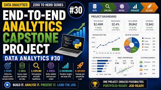
End-to-End Analytics Capstone Project | Data Analytics #30
 29 min
Lesson 10
Python Data Analytics #10: Retail Analytics Capstone — End-to-End Report in Python
 29 min
Lesson 20