 Mathew K Analytics
Lesson 11 · Real-World Data Analytics
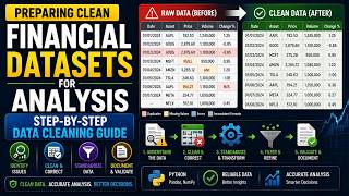
Clean Stock Price Data in Python: Apple vs Tesla with Pandas | Data Analytics #11
Real market data is messy. We load Apple and Tesla price history in pandas, fix date parsing, a malformed row and a broken volume column, then compare daily…
- CourseReal-World Data Analytics
- Lesson11 of 100
- FormatJupyter notebook · 30 code cells
- Data2 datasets
What you'll learn
Datasets used in this lesson
Save these next to the notebook. In Google Colab, upload them with the 📁 icon on the left first.
- aapl_finance_charts.csv preview58.3 KB
- tesla_stock_price.csv preview53.3 KB
📓 Full notebook
Download .ipynbData Analytics 100, Video 11: Fetching and Cleaning Real Historical Stock Price Data#
- Video eleven of the hundred-video real-world data analytics series, and the first video of Domain 2, Finance and Stock Market Analytics.
- Two real stocks, Apple and Tesla, each with real messy quirks that need real cleaning before any analysis can trust them.
- Let's get into it.
This lesson is for learners who can already load and filter a DataFrame and now want to work with financial time series. The business question is simple: once two real price histories are cleaned and lined up on the same days, which stock grew more, which was riskier, and how closely did they move together?
You work with two files. aapl_finance_charts.csv holds 506 Apple trading days with open, high, low, close, volume and adjusted price, plus moving-average bands and a direction label. tesla_stock_price.csv holds Tesla's date, close, volume, open, high and low, and it arrives with real problems: a stray intraday row, slash-formatted dates, comma-formatted volumes and reverse date order.
In this lesson you will:
- Detect and drop a malformed row with a regular expression
- Parse dates, clean a text volume column and sort chronologically
- Align two stocks on their overlapping dates with an inner merge
- Compare daily returns, volatility, correlation, cumulative growth and maximum drawdown
Prerequisites: you should be comfortable with pd.read_csv, boolean filtering and basic matplotlib plots; earlier lessons in the series cover these.
Part 1: Welcome to Domain 2, Finance and Stock Market Analytics#
This lesson opens a new domain, finance, where almost every dataset is a time series: one row per trading day. Before cleaning anything you need to know how much data you have. The code imports pandas, numpy and matplotlib, reads the Apple file with pd.read_csv, and checks .shape, which returns (rows, columns). The output is (506, 11): 506 trading days and 11 columns. Roughly 252 trading days make a market year, so this is about two years of Apple history. Make checking .shape a habit straight after every load.
import pandas as pd
import numpy as np
import matplotlib.pyplot as plt
aapl_raw = pd.read_csv('aapl_finance_charts.csv')
aapl_raw.shape
Part 2: Real Apple Data, First Look#
Before trusting any numbers you should know what type pandas assigned to each column. The code calls .head(3) and then .dtypes, but only the last expression is displayed, so the output is the list of types. Prices such as AAPL.Open and AAPL.Close are float64 and AAPL.Volume is int64, which is good. The key problem is that Date is object, meaning plain text, so you cannot sort or filter it by time yet. The direction column is also text and holds a label you will test at the end of the lesson.
aapl_raw.head(3)
aapl_raw.dtypes
Part 3: Real Apple Date Parsing#
Time series analysis only works if dates are real datetime values and rows are in time order. The code works on a .copy() so the raw data stays untouched, converts Date with pd.to_datetime, then sorts with sort_values('Date') and renumbers rows with reset_index(drop=True); drop=True throws away the old index instead of adding it as a column. The output shows the first three days start on 2015-02-17, with Apple closing at about 127.83 on that day. Always sort after parsing, because text dates can sort in the wrong order.
aapl = aapl_raw.copy()
aapl['Date'] = pd.to_datetime(aapl['Date'])
aapl = aapl.sort_values('Date').reset_index(drop=True)
aapl[['Date', 'AAPL.Open', 'AAPL.Close']].head(3)
Part 4: Real Apple Date Range and Coverage#
Knowing the exact period covered tells you what market events the data can and cannot speak to. The code computes the earliest and latest Date with .min() and .max(), then aapl.shape[0], the row count. Because Jupyter only shows the last expression, the output displays just 506, confirming no rows were lost during parsing. The min and max dates are calculated but not displayed; run that line on its own to see them. You can already tell from the previous step that the series starts in February 2015.
aapl['Date'].min(), aapl['Date'].max()
aapl.shape[0]
Part 5: Loading the Real Tesla Data#
Now you bring in the second stock, which is where the real cleaning starts. The code reads tesla_stock_price.csv, checks its shape, then shows .head(3), which is the displayed output. Three problems are visible straight away: the first row's date is 11:34, a time of day rather than a date; dates use slashes like 2018/10/15 and run newest first; and volume mixes a comma-formatted value, 4,787,699, with decimals like 6189026.0000. Spotting these in the first few rows is exactly why you always look before you analyse.
tsla_raw = pd.read_csv('tesla_stock_price.csv')
tsla_raw.shape
tsla_raw.head(3)
Part 6: Real Malformed Row in the Tesla Data#
One bad row can break date parsing for the whole column, so you need to find every row that does not look like a date. The code converts date to text with astype(str), then .str.match(r'^\d{4}/\d{2}/\d{2}$') tests each value against the pattern four digits, slash, two digits, slash, two digits, with ^ and $ meaning the whole value must match. The ~ flips the result to keep the non-matching rows. The output shows exactly one offender: the 11:34 row with a close of 270.49, which looks like an intraday snapshot rather than a daily record.
bad_rows = tsla_raw[~tsla_raw['date'].astype(str).str.match(r'^\d{4}/\d{2}/\d{2}$')]
bad_rows
Part 7: Dropping the Real Bad Row#
With only one malformed row and no date to recover it with, dropping it is the safe choice. The code applies the same regular expression without the ~, keeping only rows that match the date pattern, and adds .copy() so later edits do not trigger pandas' SettingWithCopyWarning. The output shows 756 rows remain, about three years of trading days. A good habit is to record how many rows you dropped and why, so anyone reviewing your work can follow the decision.
tsla = tsla_raw[tsla_raw['date'].astype(str).str.match(r'^\d{4}/\d{2}/\d{2}$')].copy()
tsla.shape[0]
Part 8: Real Tesla Date Parsing#
Now that every value matches one format, parsing is safe. The code uses pd.to_datetime with format='%Y/%m/%d', which tells pandas exactly how to read year, month and day. Giving an explicit format is faster and avoids pandas guessing wrongly between day-first and month-first orders. The output shows the first rows now read 2018-10-15, 2018-10-12 and 2018-10-11, with closes of 259.59, 258.78 and 252.23. Notice the index starts at 1, because the bad row 0 was removed, and the dates still run newest first.
tsla['date'] = pd.to_datetime(tsla['date'], format='%Y/%m/%d')
tsla[['date', 'close']].head(3)
Part 9: Real Volume Column Cleanup#
Volume stored as text cannot be summed or averaged, and the comma in 4,787,699 stops a direct numeric conversion. The code chains several steps: astype(str) makes every value text, .str.replace(',', '', regex=False) strips commas as a literal character, .astype(float) handles values like 6189026.0000, and .astype(int) turns them into whole numbers. Only the final head(3) is displayed, showing clean int64 values of 6,189,026, 7,189,257 and 8,128,184. Converting to float before int matters, since pandas cannot turn the text 6189026.0000 straight into an integer.
tsla['volume'].head(3)
tsla['volume'] = tsla['volume'].astype(str).str.replace(',', '', regex=False).astype(float).astype(int)
tsla['volume'].head(3)
Part 10: Real Chronological Sort#
Returns, moving averages and cumulative growth all assume rows run from oldest to newest, but the Tesla file is in reverse. The code sorts with sort_values('date') and renumbers with reset_index(drop=True). The output confirms the series now starts on 2015-10-15 with a close of 221.31, followed by 227.01 and 228.10. Forgetting this step is a classic mistake: pct_change() on reversed data gives returns with the wrong sign and timing.
tsla = tsla.sort_values('date').reset_index(drop=True)
tsla[['date', 'close']].head(3)
Part 11: Real Duplicate Date Check#
A repeated date would double count a trading day and distort returns and merges. The code uses .duplicated(), which marks every repeat after the first occurrence as True, and .sum() counts them. It checks both stocks, but only the last line, the Apple check, is displayed: 0 duplicate dates. Run the Tesla line on its own to see its count too. If you ever do find duplicates in price data, inspect them before dropping, since they can signal a data feed problem.
tsla['date'].duplicated().sum()
aapl['Date'].duplicated().sum()
Part 12: Real Date Range for Tesla#
Just as with Apple, you should confirm the time span Tesla covers. The code computes the minimum and maximum date, then the row count. Only the last expression is shown, so the output is 756 rows, matching the count after the bad row was removed. The sorted head in an earlier step showed the series begins on 2015-10-15, and the original file's first valid row was 2018-10-15, so Tesla runs roughly three years. Compare this with Apple's span before deciding how to combine them.
tsla['date'].min(), tsla['date'].max()
tsla.shape[0]
Part 13: Real Overlapping Window#
You can only compare two stocks on days where you have prices for both. The code takes the later of the two start dates with max() and the earlier of the two end dates with min(), which gives the shared window. The output shows the overlap runs from 2015-10-15 to 2017-02-16. So although Tesla data continues to 2018, any side-by-side comparison is limited to about 16 months. This max-of-starts, min-of-ends pattern works for any two date ranges.
overlap_start = max(aapl['Date'].min(), tsla['date'].min())
overlap_end = min(aapl['Date'].max(), tsla['date'].max())
overlap_start, overlap_end
Part 14: Real Merged Comparison Table#
To compare the stocks day by day you need them in one table, aligned on date. The code filters each DataFrame to the overlap window using two conditions joined with &, keeps only the date and close columns, and renames Tesla's columns to Date and TSLA.Close so the key matches. pd.merge(..., on='Date', how='inner') then keeps only dates present in both. The output shows 338 shared trading days. An inner join silently drops unmatched dates, so always check the row count afterwards.
aapl_window = aapl[(aapl['Date'] >= overlap_start) & (aapl['Date'] <= overlap_end)][['Date', 'AAPL.Close']]
tsla_window = tsla[(tsla['date'] >= overlap_start) & (tsla['date'] <= overlap_end)][['date', 'close']].rename(columns={'date': 'Date', 'close': 'TSLA.Close'})
merged = pd.merge(aapl_window, tsla_window, on='Date', how='inner')
merged.shape[0]
Part 15: Visualizing Real Apple Closing Price#
A price chart is the fastest sanity check on cleaned data: gaps, spikes or a backwards line reveal problems that summary numbers hide. The code draws Apple's closing price over its full date range with plt.plot, labels both axes, adds a title, uses tight_layout() to stop labels being cut off, then saves the figure with savefig at 120 dpi and closes it. There is no displayed output because the chart goes to a PNG file. When you open it, look for a smooth line with no sudden vertical jumps that would suggest a bad row or an unadjusted stock split.
plt.figure(figsize=(10, 5))
plt.plot(aapl['Date'], aapl['AAPL.Close'], color='steelblue')
plt.xlabel('Real Date')
plt.ylabel('Real Closing Price (USD)')
plt.title('Real Apple Closing Price History')
plt.tight_layout()
plt.savefig('aapl_price_history.png', dpi=120)
plt.close()
Part 16: Visualizing Real Tesla Closing Price#
The same check for Tesla is even more important, because this is the file you had to repair. The code plots tsla['date'] against tsla['close'] in crimson and saves it to tsla_price_history.png, so nothing is displayed inline. When you open the chart, the line should run left to right from late 2015 to late 2018 with no zigzag back in time, which would mean the sort failed. Also note how much wider Tesla's price swings look than Apple's; you will measure that properly shortly.
plt.figure(figsize=(10, 5))
plt.plot(tsla['date'], tsla['close'], color='crimson')
plt.xlabel('Real Date')
plt.ylabel('Real Closing Price (USD)')
plt.title('Real Tesla Closing Price History')
plt.tight_layout()
plt.savefig('tsla_price_history.png', dpi=120)
plt.close()
Part 17: Real Daily Returns#
Raw prices cannot be compared fairly, because a 1 dollar move means more for a cheap stock than an expensive one. Daily returns fix this by expressing each day's change as a percentage of the previous close. pct_change() computes (today minus yesterday) divided by yesterday. The first row has no previous day, so it is NaN, which is why the code uses .dropna() before showing three rows rounded to four decimals. On 2015-10-20, for example, Apple rose about 1.83% while Tesla fell about 6.61%, a first hint that they do not always move together.
merged['AAPL_Return'] = merged['AAPL.Close'].pct_change()
merged['TSLA_Return'] = merged['TSLA.Close'].pct_change()
merged[['Date', 'AAPL_Return', 'TSLA_Return']].dropna().head(3).round(4)
Part 18: Real Volatility Comparison#
Volatility measures how much a stock's returns bounce around, and analysts use it as a basic risk measure. The code takes the standard deviation of each return column with .std(), a measure of typical distance from the average, then multiplies by 100 to express it as a percentage. The output shows Apple at about 1.48% and Tesla at about 2.45% per day. In plain terms, Tesla's daily moves are typically around two thirds larger than Apple's over the same 338 days.
aapl_volatility = merged['AAPL_Return'].std()
tsla_volatility = merged['TSLA_Return'].std()
round(aapl_volatility * 100, 3), round(tsla_volatility * 100, 3)
Part 19: Real Correlation Between the Two Stocks#
Correlation tells you whether two stocks tend to rise and fall together, which matters for diversification. It runs from -1 (always opposite) through 0 (no relationship) to +1 (always together). The code builds a two-by-two correlation matrix with .corr() and picks the off-diagonal value with .iloc[0, 1]. The output is 0.217, a weak positive relationship: on average the two lean the same way, but much of each stock's movement is independent. Always correlate returns, not prices, since two trending prices can look highly correlated by accident.
return_correlation = merged[['AAPL_Return', 'TSLA_Return']].corr().iloc[0, 1]
round(return_correlation, 3)
Part 20: Real Cumulative Return Comparison#
Cumulative return answers the investor question: what would 1 dollar invested on the first shared day be worth at the end? The code replaces the first NaN return with 0 using fillna(0), adds 1 to each return to get a daily growth factor, and multiplies them together with .cumprod(). The final values, taken with .iloc[-1], are 1.21 for Apple and 1.215 for Tesla. Despite Tesla being far more volatile, both ended up roughly 21% higher over this window, which shows why return and risk must be read together.
merged['AAPL_Cumulative'] = (1 + merged['AAPL_Return'].fillna(0)).cumprod()
merged['TSLA_Cumulative'] = (1 + merged['TSLA_Return'].fillna(0)).cumprod()
round(merged['AAPL_Cumulative'].iloc[-1], 3), round(merged['TSLA_Cumulative'].iloc[-1], 3)
Part 21: Visualizing Real Cumulative Returns#
Two nearly identical end values can hide very different journeys, and a chart shows that path. The code plots both cumulative series on the same axes with labels for the legend, and plt.axhline(1, ...) draws a dashed grey line at 1, the break-even level. The figure is saved to cumulative_return_comparison.png rather than displayed. When you open it, look for how far each line dips below the dashed line and how often the two lines cross; Tesla's should look much more jagged on the way to the same finish.
plt.figure(figsize=(10, 6))
plt.plot(merged['Date'], merged['AAPL_Cumulative'], label='Real Apple')
plt.plot(merged['Date'], merged['TSLA_Cumulative'], label='Real Tesla')
plt.axhline(1, color='gray', linestyle='--')
plt.xlabel('Real Date')
plt.ylabel('Real Growth of $1 Invested')
plt.title('Real Cumulative Return, Apple vs Tesla')
plt.legend()
plt.tight_layout()
plt.savefig('cumulative_return_comparison.png', dpi=120)
plt.close()
Part 22: Saving the Real Cleaned Datasets#
Saving cleaned data means later lessons, and colleagues, start from a trusted version rather than repeating the repairs. The code writes three files with to_csv(..., index=False), which stops pandas writing the row numbers as an extra column. The merged table is rounded to four decimals with .round(4) to keep the file tidy. There is no output. A useful habit is to keep raw and clean files under clearly different names, as done here, so you never overwrite the original source.
aapl.to_csv('aapl_clean.csv', index=False)
tsla.to_csv('tsla_clean.csv', index=False)
merged.round(4).to_csv('aapl_tsla_merged.csv', index=False)
Part 23: Real Reload Verification#
Writing a file is not the same as writing it correctly, so a quick reload test is worthwhile. The code reads both cleaned CSVs back with pd.read_csv and compares their row counts with the in-memory DataFrames using ==. The output is (True, True), confirming no rows were lost in saving. Note that dates come back as text after a reload, so you would need parse_dates=['Date'] or pd.to_datetime again when you use these files in the next lesson.
reloaded_aapl = pd.read_csv('aapl_clean.csv')
reloaded_tsla = pd.read_csv('tsla_clean.csv')
reloaded_aapl.shape[0] == aapl.shape[0], reloaded_tsla.shape[0] == tsla.shape[0]
Part 24: Real Sanity Check on Cleaning#
A sanity check tests a rule that must hold if the cleaning worked. Every real trading day should have positive volume, so a zero or negative value would point to a conversion error. The code builds a True or False mask with tsla['volume'] > 0 and .all() returns True only if every value passes. The output is True. Writing small assertions like this after each cleaning step is a cheap way to catch mistakes early.
(tsla['volume'] > 0).all()
Part 25: Real Best and Worst Single Trading Days#
Extreme days show the tails of the return distribution, the moves that hurt or reward investors most. The code uses idxmax() and idxmin(), which return the row label of the largest and smallest return, then .loc to look up the matching date. The percentages are rounded and printed with an f-string, and .date() drops the time part. The output shows Apple's best day was 2016-07-27 at +6.5% and its worst was 2016-01-27 at -6.57%. Both fall in late January and late July, which is when Apple typically reports earnings.
aapl_best_day = merged.loc[merged['AAPL_Return'].idxmax(), 'Date']
aapl_worst_day = merged.loc[merged['AAPL_Return'].idxmin(), 'Date']
aapl_best_pct = round(merged['AAPL_Return'].max() * 100, 2)
aapl_worst_pct = round(merged['AAPL_Return'].min() * 100, 2)
print(f'Apple: best day {aapl_best_day.date()} at {aapl_best_pct}%, worst day {aapl_worst_day.date()} at {aapl_worst_pct}%.')
Part 26: Real Tesla Best and Worst Days#
Repeating the same logic for Tesla lets you compare how extreme each stock's tails are. The code is identical in structure, using idxmax(), idxmin() and .loc on the TSLA_Return column. The output shows Tesla's best day was 2015-11-04 at +11.17% and its worst was 2016-06-22 at -10.45%. Both extremes are well beyond Apple's roughly 6.5% moves, which is consistent with Tesla's higher volatility measured earlier.
tsla_best_day = merged.loc[merged['TSLA_Return'].idxmax(), 'Date']
tsla_worst_day = merged.loc[merged['TSLA_Return'].idxmin(), 'Date']
tsla_best_pct = round(merged['TSLA_Return'].max() * 100, 2)
tsla_worst_pct = round(merged['TSLA_Return'].min() * 100, 2)
print(f'Tesla: best day {tsla_best_day.date()} at {tsla_best_pct}%, worst day {tsla_worst_day.date()} at {tsla_worst_pct}%.')
Part 27: Real Maximum Drawdown#
Maximum drawdown is the largest fall from a previous peak to a later low, and it captures the pain an investor would actually have felt. The helper function uses .cummax() to track the highest value reached so far, computes how far each day sits below that peak as a fraction, and returns the most negative value with .min(). The output shows Apple's worst drawdown was about -26.3% and Tesla's about -40.1%. So although both ended up roughly 21% higher, a Tesla holder at one point sat on a 40% loss from the high.
def max_drawdown(cumulative):
    running_max = cumulative.cummax()
    drawdown = (cumulative - running_max) / running_max
    return drawdown.min()
round(max_drawdown(merged['AAPL_Cumulative']) * 100, 1), round(max_drawdown(merged['TSLA_Cumulative']) * 100, 1)
Part 28: Real Average Daily Volume Comparison#
Trading volume reflects how actively a stock changes hands, which affects how easily large orders can be filled. The code averages daily volume for each stock with .mean() across its full cleaned history. The output shows Apple averaged about 43,178,421 shares a day and Tesla about 6,148,865. Remember that these cover different date ranges and that share counts are not money traded, since the share prices differ, so treat this as a rough comparison of activity.
aapl_avg_volume = aapl['AAPL.Volume'].mean()
tsla_avg_volume = tsla['volume'].mean()
round(aapl_avg_volume, 0), round(tsla_avg_volume, 0)
Part 29: Real Recap Print#
A one-line summary is useful for logs, reports and anyone skimming your notebook. The code uses an f-string to insert the row counts of the three main tables. The output reads: 506 Apple trading days, 756 Tesla trading days and 338 overlapping days for direct comparison. These numbers match every earlier check, which is a good final confirmation that nothing was lost or duplicated during cleaning.
print(f'Cleaned {aapl.shape[0]} real Apple trading days and {tsla.shape[0]} real Tesla trading days; {merged.shape[0]} real days overlap for direct comparison.')
Part 30: Real Direction Column Sanity Check#
Columns you did not create yourself deserve scepticism, so this step tests the file's direction label. The code builds its own label with np.where: if the close is up or unchanged from the previous day (.diff() >= 0) it is 'Increasing', otherwise 'Decreasing'. It skips the first row, which has no previous day, and compares the two labels; .mean() on the True and False results gives the share that match. The output is about 0.814, so the labels agree on roughly 81% of days. The original column probably uses a different definition, for example close versus open, so check its documentation before relying on it.
aapl['ActualDirection'] = np.where(aapl['AAPL.Close'].diff() >= 0, 'Increasing', 'Decreasing')
(aapl['direction'].iloc[1:].values == aapl['ActualDirection'].iloc[1:].values).mean()
Wrap-Up: What You Learned#
- Real financial data pulled from the wild rarely arrives clean; comma-formatted numbers, stray malformed rows, and reversed date order are genuinely common.
- Daily percentage returns, not raw prices, are the real fair way to compare two different real stocks.
- Standard deviation of daily returns is a real standard, simple measure of volatility.
- Correlation between two real stocks' returns shows how much they genuinely move together, or don't.
- Cumulative return curves show a real intuitive answer to "what would my dollar be worth now," starting from the real same day.
- Next video: real portfolio returns, risk, and the efficient frontier, building on these exact same two real stocks.
Practice on your own
- Repeat the volatility and correlation analysis using
AAPL.Adjustedinstead ofAAPL.Closefor Apple, and check whether the volatility figure changes. - Add a 20-day rolling volatility column to
mergedwithmerged['TSLA_Return'].rolling(20).std(), plot it for both stocks and note when Tesla's risk peaked. - Redo the
directionsanity check using close versus open on the same day (aapl['AAPL.Close'] >= aapl['AAPL.Open']) and see whether the match rate rises above about 81%.
The next lesson builds on these same two cleaned stocks to look at portfolio returns, risk and the efficient frontier, so keep your saved CSV files handy.
🧠 Test yourself
Pick an answer to check it. Your best score is saved in this browser.
In the Tesla file, one row has a malformed date. How does the lesson find it?
A regular expression for the YYYY/MM/DD pattern flags rows that do not match. The ~ inverts the mask to show the bad ones.
Tesla volume arrives as text like '1,234,567'. What does the lesson do to make it numeric?
Strings with commas cannot be converted directly. Replace ',' with '' first, then cast to a number.
Why compare stocks using daily returns instead of raw closing prices?
A $300 stock and a $30 stock cannot be compared by price change in dollars. Percent returns are scale-free.
What does
(1 + returns.fillna(0)).cumprod()give you?Multiplying (1 + r) day after day compounds returns, so the final value shows what $1 would have become.
What does the lesson's
max_drawdownfunction compute with(cumulative - cumulative.cummax()) / cumulative.cummax()then.min()?cummax is the running peak. The percent below that peak is the drawdown, and its minimum is the worst decline.
💻 Practice exercises
Try each one in the notebook or in your own editor before opening the solution.
Clean this messy price table: parse the 'date' column to datetime, convert 'volume' (strings with commas) to integers, sort by date ascending, and print the result and dtypes.
💡 Hint
Use pd.to_datetime, str.replace(',', ''), and sort_values.
✅ Show solution
import pandas as pd

raw = pd.DataFrame({
    'date': ['2024/01/03', '2024/01/01', '2024/01/02'],
    'close': [11.0, 10.0, 10.5],
    'volume': ['1,200', '900', '1,050,000'],
})
df = raw.copy()
df['date'] = pd.to_datetime(df['date'], format='%Y/%m/%d')
df['volume'] = df['volume'].str.replace(',', '', regex=False).astype(int)
df = df.sort_values('date').reset_index(drop=True)
print(df)
print(df.dtypes)
Given rows where one date is malformed, keep only rows matching YYYY/MM/DD using a regex, then count duplicate dates in the cleaned data.
💡 Hint
Use .str.match(r'^\d{4}/\d{2}/\d{2}$') as a boolean mask.
✅ Show solution
import pandas as pd

raw = pd.DataFrame({
    'date': ['2024/01/01', '2024/01/02', 'bad-row', '2024/01/02', '2024/01/03'],
    'close': [10, 11, 0, 11, 12],
})
mask = raw['date'].astype(str).str.match(r'^\d{4}/\d{2}/\d{2}$')
print('Bad rows:')
print(raw[~mask])
clean = raw[mask].copy()
clean['date'] = pd.to_datetime(clean['date'], format='%Y/%m/%d')
print('Duplicate dates:', clean['date'].duplicated().sum())
Make two synthetic price series of 120 business days (seeds 1 and 2, start 100, daily percent moves normal with mean 0.0005 and std 0.01). Merge them on date, compute daily returns, print each volatility (std of returns, in %), the return correlation, the final growth of $1 for each, and the max drawdown of the first.
💡 Hint
Use pct_change, cumprod, and cummax as in the lesson.
✅ Show solution
import numpy as np
import pandas as pd

dates = pd.bdate_range('2024-01-01', periods=120)
def make(seed):
    r = np.random.default_rng(seed).normal(0.0005, 0.01, 120)
    return pd.Series(100 * np.cumprod(1 + r), index=dates)

merged = pd.DataFrame({'A': make(1), 'B': make(2)})
rets = merged.pct_change().dropna()
print('Volatility %:', (rets.std() * 100).round(3).to_dict())
print('Correlation:', round(rets['A'].corr(rets['B']), 3))

cum = (1 + rets).cumprod()
print('Final growth:', cum.iloc[-1].round(3).to_dict())

def max_drawdown(c):
    return ((c - c.cummax()) / c.cummax()).min()
print('Max drawdown A %:', round(max_drawdown(cum['A']) * 100, 1))
Found this useful?
All lessons, notebooks and datasets here are free. If they helped you, a coffee keeps new lessons coming.
Related lessons
 23 min
Clean Stock Market Data in Python: yfinance + pandas Guide
 15 min
Building a House Price Prediction Model with Python: Data Science and Machine Learning
 26 min
Data Mining with Python: pandas & scikit-learn Crash Course
 19 min